Unveiling the Ultimate Secret of High Concurrency: How Java Thrives in High-Frequency Trading?

The Characteristics of High-Frequency Trading Systems

In the current financial markets, there is a significant need for high-frequency trading (HFT) systems. Java, renowned for its cross-platform compatibility, efficient development capabilities, and maintainable features, is extensively employed within the financial industry. High-frequency trading revolves around the rapid execution of buy and sell transactions, leveraging swift algorithms and advanced computer technology, all while prioritizing the attainment of low-latency targets.

The Challenges: High Concurrency Processing and Low Latency Requirements

High-frequency trading systems necessitate managing many trade requests within extremely tight timeframes, creating substantial demands for robust concurrency processing capabilities and exceptional low-latency performance.

How can the challenges of high concurrency and low latency be tackled?

Conventional data structures and algorithms may be inadequate to meet high-frequency trading systems’ high concurrency and low latency demands. As a result, exploring more efficient concurrent data structures becomes imperative.

Limitations of Traditional Queues in High-Frequency Trading Systems

Traditional queue data structures, such as LinkedList, ArrayBlockingQueue, and ConcurrentLinkedQueue, face limitations in high-frequency trading systems. These queues may encounter issues like lock contention, thread scheduling overhead, and increased latency, preventing them from meeting high-frequency trading requirements. The lock and synchronization mechanisms in traditional queues introduce additional overhead, restricting their ability to efficiently handle high concurrency and achieve low-latency performance.

The limitations of traditional queues in high-frequency trading systems can be summarized as follows:

  1. Lock contention: Traditional queues use locks to ensure thread safety during concurrent access. However, when many threads compete for locks simultaneously, performance can degrade, and latency can increase. Locks introduce extra overhead, potentially leading to thread blocking and extended system response times.
  2. Thread scheduling overhead: In traditional queues, frequent thread scheduling operations occur when threads wait or are awakened within the queue. This overhead adds to system costs and introduces additional latency. Frequent thread context switching in high-concurrency scenarios can waste system resources and degrade performance.
  3. Increased latency: Due to issues like lock contention and thread scheduling, traditional queues may fail to meet the low-latency requirements of high-frequency trading systems in high-concurrency environments. Trade requests waiting in the queue experience increased processing time, resulting in longer trade execution times and affecting real-time responsiveness and system performance.

These limitations prevent the standard queues provided by the JDK from meeting the high concurrency processing and low-latency performance requirements of high-frequency trading systems. To address these issues, it is necessary to explore more efficient concurrent data structures, such as the Disruptor, to overcome the challenges posed by high-frequency trading systems.

Introduction to the Disruptor Framework

Disruptor is a high-performance concurrent data structure developed by LMAX Exchange. It aims to provide a solution with high throughput, low latency, and scalability to address concurrency processing challenges in high-frequency trading systems.

Core Concepts and Features of Disruptor

Disruptor tackles concurrent challenges through core concepts such as the ring buffer, producer-consumer model, and lock-free design. Its notable features include:

  1. High Performance: Disruptor’s lock-free design minimizes competition and overhead among threads, resulting in exceptional performance.
  2. Low Latency: Leveraging the ring buffer and batch processing mechanism, Disruptor achieves extremely low latency, meeting the stringent requirements of high-frequency trading systems.
  3. Scalability: Disruptor’s design allows effortless expansion to accommodate multiple producers and consumers while maintaining excellent scalability.

Ring Buffer

The Ring Buffer is a core component of the Disruptor framework. It is a circular buffer for efficient storage and transfer of events or messages, enabling high-performance and low-latency data exchange between producers and consumers.

Key Features of Disruptor’s Ring Buffer:

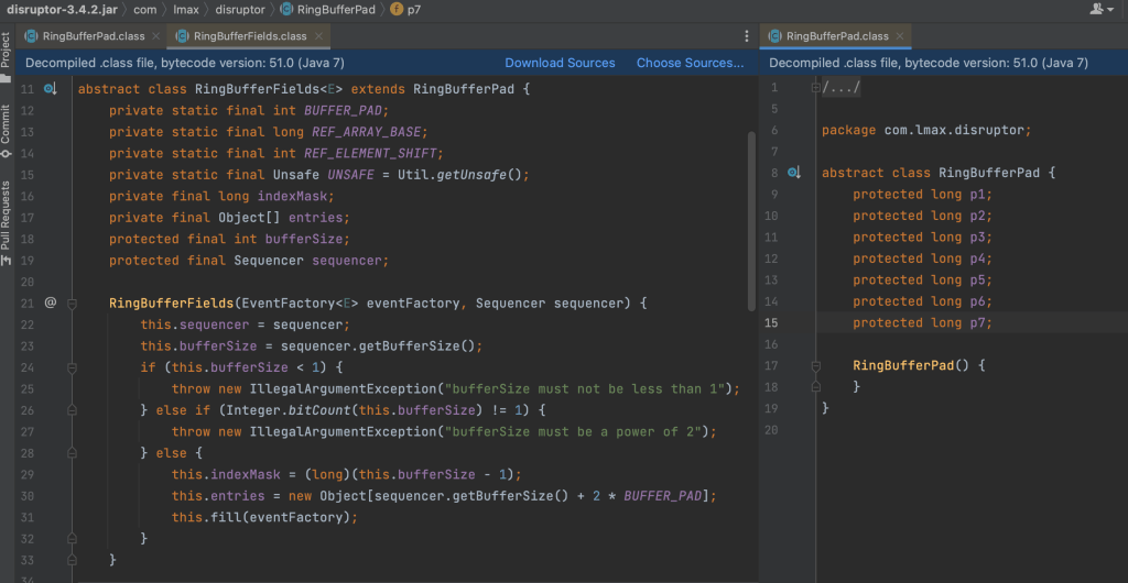
Cache Line Optimization

Disruptor is designed to leverage cache line utilization for improved access efficiency. By placing padding data in the same cache line, unnecessary cache contention and cache invalidation are minimized, resulting in enhanced read and write performance.


The following code demonstrates how to improve performance by using padding data placement.

import java.util.concurrent.CountDownLatch;

public class CacheLinePadding {
    public static volatile long COUNT = 10_0000_0000L;

    private static abstract class TestObject {
        public long x;
    }

    private static class Padded extends TestObject {
        public volatile long p1, p2, p3, p4, p5, p6, p7;
        public long x;
        public volatile long p9, p10, p11, p12, p13, p14, p15;
    }

    private static class Unpadded extends TestObject {
        // Empty class, no padding required
    }

    public static void runTest(boolean usePadding) throws InterruptedException {
        TestObject[] arr = new TestObject[2];
        CountDownLatch latch = new CountDownLatch(2);

        if (usePadding) {
            arr[0] = new Padded();
            arr[1] = new Padded();
        } else {
            arr[0] = new Unpadded();
            arr[1] = new Unpadded();
        }

        Thread t1 = new Thread(() -> {
            for (long i = 0; i < COUNT; i++) {
                arr[0].x = i;
            }
            latch.countDown();
        });

        Thread t2 = new Thread(() -> {
            for (long i = 0; i < COUNT; i++) {
                arr[1].x = i;
            }
            latch.countDown();
        });

        long start = System.nanoTime();
        t1.start();
        t2.start();
        latch.await();
        System.out.println((usePadding ? "Test with padding: " : "Test without padding: ") +
                (System.nanoTime() - start) / 100_0000);
    }

    public static void main(String[] args) throws Exception {
        runTest(true);  // Test with padding
        runTest(false); // Test without padding
    }
}

Here’s the result:

Test with padding: 738
Test without padding: 2276

Similar Implementation in the Disruptor Framework

Circular Buffer Structure

Disruptor utilizes a circular buffer as its primary data structure, providing efficient event storage and delivery. Using a circular buffer eliminates the need for dynamic memory allocation and resizing, optimizing overall performance.

Strict Ordering

Disruptor ensures events are consumed in the same order they were produced, maintaining data flow integrity and consistency.

Lock-Free Design and CAS Operations

Disruptor employs a lock-free design and atomic operations, such as Compare-and-Swap (CAS), to achieve high concurrency. This reduces thread contention and enhances concurrent processing capabilities.

For a detailed understanding of how CAS (Compare and Swap) operates and its application in addressing high concurrency challenges, I recommend referring to my previous article available at: https://masteranyfield.com/2023/07/03/unleashing-the-potential-of-synchronized-and-cas-addressing-high-concurrency-challenges-in-e-commerce-and-hft/.

High Performance and Low Latency

By leveraging the circular buffer and batch processing mechanisms, Disruptor achieves exceptional performance and ultra-low latency. It meets the stringent low-latency requirements of high-frequency trading systems.

Scalability

Disruptor’s design allows for easy scalability to accommodate multiple producers and consumers, providing flexibility to handle increasing thread and processing demands.

Disruptor VS Traditional Queues

Disruptor offers significant advantages over standard JDK queues in terms of low latency, scalability, and high throughput:

  1. Low Latency: Disruptor is designed to achieve low-latency data processing. By minimizing lock contention, reducing thread context switching, and leveraging the ring buffer structure, Disruptor provides extremely low event processing latency. This makes it highly suitable for applications with strict real-time requirements, such as high-frequency trading systems.
  2. Scalability: Disruptor employs a lock-free design and efficient concurrent algorithms, allowing it to effortlessly scale to accommodate multiple producers and consumers. This enables Disruptor to handle large-scale concurrent operations while maintaining high performance and scalability.
  3. High Throughput: Disruptor achieves exceptional throughput through optimized design and lock-free mechanisms. Multiple producers and consumers can operate in parallel by utilizing the ring buffer and implementing batch processing, maximizing system throughput.

Disruptor is well-suited for scenarios with high concurrency and demanding low latency, while traditional queues are suitable for general concurrency requirements.

Comparing Disruptor Performance with LinkedBlockingQueue and ArrayBlockingQueue

import com.lmax.disruptor.*;
import com.lmax.disruptor.dsl.Disruptor;
import com.lmax.disruptor.dsl.ProducerType;

import java.util.concurrent.*;

/**
 * Author: Adrian LIU
 * Date: 2020-07-18
 * Desc: Compare the difference of performance between Disruptor, LinkedBlockingQueue and ArrayBlockingQueue
 * implemented Producer and Consumer with single producer and consumer
 * Disruptor took 137ms to handle 10000000 tasks
 * ArrayBlockingQueue took 2113ms to handle 10000000 tasks
 * LinkedBlockingQueue took 1312ms to handle 10000000 tasks
 */
public class DisruptorVSBlockingQueueWithSingleProducerConsumer {
    private static final int NUM_OF_PRODUCERS = 1;
    private static final int NUM_OF_CONSUMERS = 1;
    private static final int NUM_OF_TASKS = 10000000;
    private static final int BUFFER_SIZE = 1024 * 1024;

    public static void main(String[] args) {
        LongEventFactory factory = new LongEventFactory();
        ExecutorService service1 = Executors.newCachedThreadPool();
        SimpleTimeCounter disruptorTimeCount = new SimpleTimeCounter("Disruptor", NUM_OF_PRODUCERS + 1, NUM_OF_TASKS);

        Disruptor<LongEvent> disruptor = new Disruptor<LongEvent>(factory, BUFFER_SIZE, service1, ProducerType.SINGLE, new SleepingWaitStrategy());
        LongEventHandler handler = new LongEventHandler(NUM_OF_TASKS, disruptorTimeCount);

        disruptor.handleEventsWith(handler);

        disruptor.start();
        RingBuffer<LongEvent> ringBuffer = disruptor.getRingBuffer();

        LongEventTranslator translator = new LongEventTranslator();

        disruptorTimeCount.start();
        new Thread(() -> {
            for (long i = 0; i < NUM_OF_TASKS; i++) {
                ringBuffer.publishEvent(translator, i);
            }

            disruptorTimeCount.count();
        }).start();

        disruptorTimeCount.waitForTasksCompletion();
        disruptorTimeCount.timeConsumption();
        disruptor.shutdown();
        disruptor.shutdown();
        service1.shutdown();

        SimpleTimeCounter arrayQueueTimeCount = new SimpleTimeCounter("ArrayBlockingQueue", NUM_OF_CONSUMERS, NUM_OF_TASKS);
        BlockingQueue<LongEvent> arrayBlockingQueue = new ArrayBlockingQueue<>(BUFFER_SIZE);

        LongEvent poisonPill = new LongEvent(-1L);
        LongEventProductionStrategy productionStrategy = new LongEventProductionStrategy(0, NUM_OF_TASKS, poisonPill, NUM_OF_CONSUMERS);
        LongEventConsumptionStrategy consumptionStrategy = new LongEventConsumptionStrategy(poisonPill, arrayQueueTimeCount);

        Thread t1 = new Thread(new BlockingQueueProducer<>(arrayBlockingQueue, productionStrategy));
        Thread t2 = new Thread(new BlockingQueueConsumer<>(arrayBlockingQueue, consumptionStrategy));
        t2.start();

        arrayQueueTimeCount.start();
        t1.start();

        arrayQueueTimeCount.waitForTasksCompletion();
        arrayQueueTimeCount.timeConsumption();

        SimpleTimeCounter linkedQueueTimeCount = new SimpleTimeCounter("LinkedBlockingQueue", NUM_OF_CONSUMERS, NUM_OF_TASKS);
        BlockingQueue<LongEvent> linkedBlockingQueue = new LinkedBlockingQueue<>();

        try {
            t1.join();
            t2.join();
        } catch (InterruptedException e) {
            e.printStackTrace();
        }

        consumptionStrategy = new LongEventConsumptionStrategy(poisonPill, linkedQueueTimeCount);
        t1 = new Thread(new BlockingQueueProducer<>(linkedBlockingQueue, productionStrategy));
        t2 = new Thread(new BlockingQueueConsumer<>(linkedBlockingQueue, consumptionStrategy));
        t2.start();

        linkedQueueTimeCount.start();
        t1.start();

        linkedQueueTimeCount.waitForTasksCompletion();
        linkedQueueTimeCount.timeConsumption();
    }
}
Disruptor took 137ms to handle 10000000 tasks
ArrayBlockingQueue took 2113ms to handle 10000000 tasks
LinkedBlockingQueue took 1312ms to handle 10000000 tasks

Based on our experiments and explanations above, it is evident that Disruptor exhibits significant advantages over the standard JDK Queue in certain scenarios. Its features, such as low latency, high throughput, concurrency, and scalability, effectively address challenges encountered in high-frequency trading (HFT) and other demanding environments.

Here are some of its applications in Fintech and trading systems:

  1. Trade Data Aggregation: Disruptor’s high throughput and low latency make it ideal for rapidly aggregating and processing large volumes of trade data. It efficiently handles numerous trade requests and ensures real-time and accurate processing.
  2. Event-Driven Trade Execution: With an event-driven model, Disruptor enables efficient concurrent processing by allowing producers to publishing trade events and consumers to execute the corresponding trade logic. This eliminates performance bottlenecks associated with traditional lock mechanisms, enabling swift trade execution and prompt response to market changes.
  3. Parallel Computing and Risk Management: Disruptor’s scalability and concurrent processing capabilities facilitate efficient handling of large-scale computing tasks and effective risk management in high-frequency trading. By leveraging Disruptor’s parallel computing capabilities, accurate risk assessment and trade decision execution can be achieved.
  4. Lock-Free Design and Low Latency: Disruptor’s lock-free design minimizes lock contention and thread scheduling overhead, resulting in low-latency data exchange and processing. This meets the high-concurrency and low-latency requirements of HFT, enabling rapid response to market changes and improved trade execution efficiency.

Summary

Disruptor’s exceptional features, including low latency, high throughput, concurrency, and scalability, empower HFT systems to overcome challenges and achieve faster and more efficient trade execution. Its applications in trade data aggregation, event-driven trade execution, parallel computing, risk management, and lock-free design contribute to its effectiveness in high-frequency trading systems.

Unleashing the Java Concurrent Potential: Conquering High-Concurrency Challenges with Optimal Adoption of Synchronized and CAS

Synchronized and Compare and Swap (CAS) are two major concurrent mechanisms in Java used to solve thread safety issues. Choosing the appropriate mechanism can significantly improve the performance and resource utilization of your Java application.

In terms of features, synchronized is a keyword provided by Java, while CAS has its own set of implementations, such as AtomicLong and several classes that utilize AbstractQueuedSynchronizer (AQS), such as ReentrantLock and ReentrantReadWriteLock.

This article will delve into their respective advantages and disadvantages through the following structure to help us make informed choices.

Basic features and usage

Synchronized mainly controls the granularity of locks in three ways:

public class SynchronizedVSLock {
    private Object lock = new Object();

    public void objectLock() {
        // The lock is scoped to the code block below, ensuring exclusive access within that block.
        synchronized (lock) {

        }
    }

    public void classLock() {
        // The code block is protected by a global lock associated with the SynchronizedVSLock.class, ensuring that concurrent access by any instances is synchronized.
        synchronized (SynchronizedVSLock.class) {

        }
    }

    // The lock is scoped to the method, ensuring exclusive access within its execution.
    public synchronized void methodLock() {

    }
}

In contrast, Lock controls the lock granularity through the lock() and unlock() methods and its scope depends on the lifecycle of the lock instance:

public class SynchronizedVSLock {
    private Lock reentrantLock = new ReentrantLock();

    public void raceConditionDemo() {
        reentrantLock.lock();
        // critical area
        reentrantLock.unlock();
    }
}

Synchronized releases the lock passively only after executing the synchronized code block or when an exception occurs. It cannot provide non-blocking lock acquisition methods.

On the other hand, Lock is more flexible than synchronized. It allows autonomous decisions on when to lock and unlock. The tryLock() method can be used to acquire a boolean value, indicating whether the lock is already held by another thread. Additionally, Lock provides both fair and unfair locks, while synchronized only provides unfair locks.

Performance comparison

Synchronized has different lock states during its implementation, including no lock, biased lock, lightweight lock, and heavyweight lock. When it is upgraded to a heavyweight lock, system calls and context switching occurs, resulting in significant performance overhead.

Java threads are mapped to native operating system threads, and blocking or waking up a thread involves a context switch between user mode and kernel mode. This switch consumes system resources and requires overhead for passing variables and parameters between modes. The kernel preserves register values and variables during the mode transition.

Frequent thread state transitions can consume a significant amount of CPU processing time. In cases where the time spent on context switching due to a heavyweight lock exceeds the time spent on executing user code, this synchronization strategy becomes highly inefficient.

When is synchronized applicable?

In contrast to the previous point, the synchronized keyword is suitable when the time taken to acquire the heavyweight lock is shorter than the time spent on executing user code. This is particularly true in scenarios where multiple threads spin and compete for resources that require a significant duration of execution. After all, spinning also occupies CPU time slices.

CAS principle

CAS (Compare and Swap) is a commonly used atomic operation in concurrent programming to address race conditions in a multi-threaded environment. The CPU primitive for CAS is the Lock cmpxchg instruction. The usage of “Lock” ensures atomicity during the comparison and write phase, preventing concurrency issues. The Lock cmpxchg instruction locks the memory block during the CAS operation, disallowing access from other CPUs.

The CAS principle involves the following key steps:

  • Comparison: CAS compares the value in memory with the expected value. If they match, it proceeds to the next step. Otherwise, another thread has modified the value, resulting in a failed CAS operation.
  • Exchange: If the comparison succeeds, CAS attempts to write the new value into memory. This operation is atomic, ensuring it is not interfered with by other threads.
  • Check result: CAS returns a boolean indicating the success or failure of the operation.

CAS is based on the atomicity of comparison and exchange operations. By comparing the value in memory with the expected value, CAS ensures only one thread successfully executes the operation. In multi-threaded scenarios, CAS maintains data consistency and correctness.

Performance comparison of synchronized and CAS implementations in different scenarios

Comparison of synchronized, AtomicLong, and LongAdder:

import java.util.concurrent.atomic.AtomicLong;
import java.util.concurrent.atomic.LongAdder;

public class AtomicVsSyncVsLongAdder {
    private static int NUM_OF_THREADS = 100;
    private static long COUNT = 0L;
    private static AtomicLong atomicLong = new AtomicLong();
    private static LongAdder longAdder = new LongAdder();

    public static void main(String args[]) throws InterruptedException {
        Thread[] threads = new Thread[NUM_OF_THREADS];

        for (int i = 0; i < threads.length; i++) {
            threads[i] = new Thread(() -> {
                for (int k = 0; k < 100000; k++) {
                    synchronized (AtomicVsSyncVsLongAdder.class) {
                        COUNT++;
                    }
                }
            });
        }

        long startTime = System.currentTimeMillis();
        for (int i = 0; i < threads.length; i++) {
            threads[i].start();
        }

        for (int i = 0; i < threads.length; i++) {
            threads[i].join();
        }
        long expiredTime = System.currentTimeMillis();

        System.out.println("Synchronized took " + (expiredTime-startTime) + "ms.");

        for (int i = 0; i < threads.length; i++) {
            threads[i] = new Thread(() -> {
                for (int k = 0; k < 100000; k++) {
                    atomicLong.incrementAndGet();
                }
            });
        }

        startTime = System.currentTimeMillis();
        for (int i = 0; i < threads.length; i++) {
            threads[i].start();
        }

        for (int i = 0; i < threads.length; i++) {
            threads[i].join();
        }
        expiredTime = System.currentTimeMillis();

        System.out.println("AtomicLong took " + (expiredTime-startTime) + "ms.");

        for (int i = 0; i < threads.length; i++) {
            threads[i] = new Thread(() -> {
                for (int k = 0; k < 100000; k++) {
                    longAdder.increment();
                }
            });
        }

        startTime = System.currentTimeMillis();
        for (int i = 0; i < threads.length; i++) {
            threads[i].start();
        }

        for (int i = 0; i < threads.length; i++) {
            threads[i].join();
        }
        expiredTime = System.currentTimeMillis();

        System.out.println("LongAdder took " + (expiredTime-startTime) + "ms.");
    }
}

When NUM_OF_THREADS is set to 100, the test results are as follows:

Synchronized took 981ms.
AtomicLong took 680ms.
LongAdder took 74ms.

When NUM_OF_THREADS is set to 1000, the test results are as follows:

Synchronized took 4472ms.
AtomicLong took 6958ms.
LongAdder took 157ms.

The experiments demonstrate that as the number of competing threads increases, the AtomicLong implementation based on CAS takes longer than the synchronized mechanism. This confirms the considerations mentioned earlier:

  • CAS can be considered when lock acquisition time is shorter than code execution time.
  • When there is high thread contention and the overhead of spinning exceeds suspension costs, using the synchronized keyword is advisable.

Spring Boot + AWS Aurora MySQL Read Write Segregation

MySQL Read write segregation brings a great amount of benefits to our applications in terms of performance and stress resistance. These includes:

  1. The capability of query process increase as the number of physical machines increase;
  2. The reader and writer response for read and write respectively greatly alleviates exclusive lock and share lock contention;
  3. We can independently improve and optimize the read, e.g. using myiasm engine setting with specific optimization parameters;
  4. Synchronization via binlog;
  5. Improve availability.

AWS Aurora has made read write segregation really simple.

In the following section, I will explain how to write a SpringBoot application to work with Aurora reader and writer. We will first create the Aurora cluster then writing an annotation to enable classes or methods to use reader or writer as data source.

Step 1: create an Aurora cluster with reader and writer

Step 2: The Spring Boot application configuration

spring:
  datasource:
    reader:
      username: admin
      password: [your_password]
      driver-class-name: com.mysql.cj.jdbc.Driver
      jdbc-url: jdbc:mysql://your_reader_url:3306/commentdb?serverTimezone=UTC&useUnicode=true@characterEncoding=utf-8
      pattern: get*,find*
    writer:
      username: admin
      password: [your_password]
      driver-class-name: com.mysql.cj.jdbc.Driver
      jdbc-url: jdbc:mysql://your_writer_url:3306/commentdb?serverTimezone=UTC&useUnicode=true@characterEncoding=utf-8
      pattern: add*,update*
  jpa:
    hibernate:
      ddl-auto: update

server:
  port: 8080

Step 3: The Dynamic Data Source

We will extends the AbstractRoutingDataSource class to write our dynamic data source

public class DynamicDataSource extends AbstractRoutingDataSource {
    public DynamicDataSource(DataSource defaultTargetDataSource, Map<Object, Object> targetDataSources) {
        super.setDefaultTargetDataSource(defaultTargetDataSource);
        super.setTargetDataSources(targetDataSources);
        super.afterPropertiesSet();
    }

    @Override
    protected Object determineCurrentLookupKey() {
        return DynamicDataSourceContextHolder.getDataSourceType();
    }
}

We will have a DynamicDataSourceContextHolder class internally using ThreadLocal to ensure

every thread has its own data source context which won’t be changed by other threads.

public class DynamicDataSourceContextHolder {
    /**
     * Use ThreadLocal to make sure every thread has its own data source context
     * which won't be changed by other threads
     */
    private static final ThreadLocal<String> CONTEXT_HOLDER = new ThreadLocal<>();

    public static void setDataSourceType(String dataSourceType){
        CONTEXT_HOLDER.set(dataSourceType);
    }

    public static String getDataSourceType(){
        return CONTEXT_HOLDER.get();
    }

    public static void clearDataSourceType(){
        CONTEXT_HOLDER.remove();
    }
}

Step 4: The DataSource annotation

We will have a DataSource annotation, which can annotate both classes and methods.

Here’s how it works:

  1. If a class is annotated with @DataSource, all its methods matches the regex rules we specify in our application.properties will switch to their related datasource.
  2. If both a method and its class are annotated with @DataSource, only the method annotation will take effect.

The DataSourceType enum

public enum DataSourceType {
    READER,
    WRITER
}

The DataSource Annotation

@Target({ ElementType.METHOD, ElementType.TYPE})
@Retention(RetentionPolicy.RUNTIME)
@Documented
public @interface DataSource {
    DataSourceType value() default DataSourceType.WRITER;
}

The DataSourceAspect

@Aspect
@Order(1)
@Component
public class DataSourceAspect {
    private final Pattern READ_PATTERN;
    private final Pattern WRITER_PATTERN; // by default we use writer

    public DataSourceAspect(@Value("${spring.datasource.reader.pattern}") String readPattern,
                            @Value("${spring.datasource.writer.pattern}") String writerPattern) {
        READ_PATTERN = Pattern.compile(getRegex(readPattern));
        WRITER_PATTERN = Pattern.compile(getRegex(writerPattern));
    }

    private String getRegex(String str) {
        return str.replaceAll("\\*", ".*")
                                 .replaceAll(" ", "")
                                 .replaceAll(",", "|");
    }

    @Around("within(@com.osfocus.springbootreadwritesegregation.annotation.DataSource *)")
    public Object around(ProceedingJoinPoint point) throws Throwable {
        MethodSignature signature = (MethodSignature) point.getSignature();
        point.getTarget();
        Method method = signature.getMethod();
        DataSource dataSource = method.getAnnotation(DataSource.class);
        if (dataSource != null) {
            // In order to have higher granularity,
            // I make method level annotation has higher priority than the class level.
            DynamicDataSourceContextHolder.setDataSourceType(dataSource.value().name());
        } else {
            if (READ_PATTERN.matcher(method.getName()).matches()) {
                DynamicDataSourceContextHolder.setDataSourceType(DataSourceType.READER.name());
            } else {
                DynamicDataSourceContextHolder.setDataSourceType(DataSourceType.WRITER.name());
            }
        }

        try {
            return point.proceed();
        } finally {
            // clear data source after method's execution.
            DynamicDataSourceContextHolder.clearDataSourceType();
        }
    }
}

We will have Comment related Controller, Service and Repository to simulate requests to read, update and write comments to social media platforms.

We annotate the CommentServiceImpl service

@Service
@DataSource
public class CommentServiceImpl implements CommentService {
    @Autowired
    private CommentRepository commentRepository;

    public List<Comment> findTop25() {
        return commentRepository.findTop25ByOrderByIdDesc();
    }

    public void addComment(CommentDTO commentDTO) {
        commentRepository.save(Comment.builder()
                                      .content(commentDTO.getContent())
                                      .build());
    }

    public void updateLastComment(CommentDTO commentDTO) {
        Optional<Comment> lastCommentOpt = commentRepository.findTopByOrderByIdDesc();
        if (lastCommentOpt.isPresent()) {
            commentRepository.updateLastComment(lastCommentOpt.get().getId(), commentDTO.getContent());
        }
    }
}

Last Step: The JMeter test

Without Read/Write segregation

With Read/Write Segregation enable

As we can see from the above two screenshots of the simple experiment, there’s improvement on the throughput.

In the experiment, the db instances are still way below its upper capability and they used the default parameter groups. As an extra machine involved, its capability of handling queries is certain to have dramatically improvement. Also, we can play around with the parameter group to make its performance better.

Here’s the code: https://github.com/adrianinthecloud/spring-aurora-read-write-segregation

Have fun.

Keep your services healthy with circuit-breaker

The circuit-breaker is not that much different from Stop Loss in stock investment.

When your Titanic has leaking holes, the entire ship will sink if you don’t have another protection layer to isolate those leaking holes.

The essence of Circuit-breaker is to isolate unavailable dependent services to avoid cascaded service unavailability.

Typical issues caused by bad dependent services

  1. Exhausting resource because of dependent service late response or no response for a long period.
    • Ever request will open certain resource in a server. The threads will be locked until the request is timeout. In high concurrent scenario, it could exhaust the server’s resource.
    • If microservice applications run on containers, this could lead to the container got killed because run out of memory.
  2. Causing MQ unavailability. If two services are interacted with each other using ActiveMQ. Service A keeps sending message to the ActiveMQ while Service B is unavailable. This could result in the ActiveMQ runs out of storage such as too much message in the DLQ. And finally, the MQ becomes unavailable.

The Circuit-Breaker Design

Other implementations, frameworks, design and approaches will be provided when I have time.

GCs of JVM tuning: PS+PO VS CMS VS G1

When it comes to GCs of JVM tuning, the following important concepts have to be elaborated:

STW(Stop the world)

The GC pause in which all business threads stop to reach to the safe point.

Take dining in a restaurant as an example, the waiters need to wait till customers finish certain meals before collecting those garbage, otherwise, it could mess up things. It’s same here for GC. At certain phrases of garbage collection, we will need the safe point, like customers stop dining, to collect garbage.

Response time

The shorter the STW, the better the response time. Websites and APIs normally need to optimise the response time. CMS and G1 are the GCs for response time first application.

Throughput

throughput = business logic execution time / (business logic execution time + GC time)

Data mining, compute-intensive applications and schedule tasks modules are typical examples of throughput first application. Parallel Scavenge and Parallel Old are for throughput focus application. It has approximately 10-15% higher throughput compared to G1 in certain scenarios.

Before getting in deep of these three typical GCs, let’s start with some basic important concepts.

Reference count and Root-finding algorithms

Reference count(RC) use the number of reference that objects have to determine whether to collect them. The problem is circular reference.

From the above diagram, ObjA, ObjB and ObjC are all have 1 reference count. However, they are not live objects and supposed to be collected. This is the circular reference problem of RC. The GC won’t collect them if it is based upon the condition of only collect if reference count equals to 0.

Root-finding

This algorithm starts from the roots of the application program.

  • GC Roots include
  • Stack Local variables, run-time methods variables
  • static variables and constants
  • class objects referenced by run-time constant pool
  • objects referred by JNI
  • Objects used as synchronized monitor.

From these root, the algorithm will find out all reachable objects, and these objects are uncollectible objects.

Three common GC algorithms

Mark-Sweep

The mark-sweep algorithm marks and collects those collectable blocks.

Pros:

  1. It is effective when there are many live objects and small amount of collectable objects;
  2. It is suitable for tenured region.
  3. CMS uses this algorithm.

Cons:

  1. It is relatively low efficiency as it will need to scan twice for the entire region.
    1. First scan to find out those live objects;
    2. Second scan to find those collectable objects for collection.
  2. It will generate memory fragments.
  3. It is not suitable for Eden region as there are small amount of live objects.

Copy

The copy algorithm divides the target region memory into two part. It copies all live objects to the second part and clean up the first part.

Pros:

  1. It does not generate memory fragments.
  2. It only need to scan once, relatively high efficiency for small amount of live objects.
  3. It is suitable for Eden region.

Cons:

  1. It wastes half of the region memory.
  2. It will need to adjust object references because it moves objects around.

Mark-Compact

The mark-compact algorithm marks and moves all live objects to the beginning of the region.

Pros:

  1. It won’t generate memory fragments.
  2. It is good for objects’ allocation.
  3. It won’t cause the waste of memory.

Cons:

  1. It is relatively low performance, because it needs to scan twice and compacts objects.
  2. Synchronisation is required when multi threads invoked.

Garbage Collectors

Parallel Scavenge and Parallel Old

Parallel Scavenge(PS) is a stop-the-world, copying collector using multiple GC threads.

Parallel Old(PO) is a stop-the-world, compacting collector using multiple GC threads.

They work together to deal with young and old generation respectively.

This combination is good for throughput-prioritised applications.

Common Parameters of PS + PO:

-XX:SurvivorRatio
-XX:PreTenureSizeThreshold
-XX:MaxTenuringThreshold (in JDK 8, the maximum value is 15 because only 4 bits to store this value in class file)
-XX:TargetSurvivorRatio (this is the parameter that actually determines whether objects should promoted to the tenured region or not.)
-XX:+ParallelGCThreads
-XX:+UseAdaptiveSizePolicy
In-depth understanding of XX:TargetSurvivorRatio
uint ageTable::compute_tenuring_threshold(size_t survivor_capacity) {
  size_t desired_survivor_size = (size_t)((((double) survivor_capacity)*TargetSurvivorRatio)/100);
  size_t total = 0;
  uint age = 1;
  assert(sizes[0] == 0, "no objects with age zero should be recorded");
  while (age < table_size) {
    total += sizes[age];
    // check if including objects of age 'age' made us pass the desired
    // size, if so 'age' is the new threshold
    if (total > desired_survivor_size) break;
    age++;
  }
  uint result = age < MaxTenuringThreshold ? age : MaxTenuringThreshold;

From the above C++ code snippet, we can see that the TargetSurvivorRatio flag is the actually parameter that determines whether objects should promoted to the tenured region or not. Basically, it sums up total size between 0 to specific age, that is just understand the ratio threshold and other objects with age above the threshold will be promoted.

ParNew and Concurrent Mark Sweep(CMS)

ParNew is kinda like the new version of PS with extra feature and enhancement. Its enhancement allows it to work with CMS. For example, it satisfies the synchronisation need during the concurrent phases of CMS.

CMS is a revolutionary GC designed to target small amount memory (from hundreds of MB to several GB) with low pause. It realises the concurrent operation of GC and business threads.

ParNew + CMS + Serial Old are worked as a combination.

Card Table

When YGC occurs, scanning the all objects in the tenured region is unnecessary overhead. Therefore, CMS has a the card table mechanism to save the unnecessary overhead.

It a divide and conquer approach. The card table uses cards to mark chunks of the old region. Each card contains multiple objects. When the application starts, the card table works with write barrier to monitor those cross-region reference. The write barrier is not memory fence. It works like AOP in spring. When assignment happens to a reference, it will change the card table, e.g. CARD_TABLE[this address >> 9] = 0. Those cards with cross-region references are marked as dirty so that during YGC, the GC only need to scan those dirty cards rather than all objects in the old region.

Tri-Color Marking Algorithm

Black, grey and white colours are used for marking objects.

Objects marked with black colour means itself and all objects it refer to have been scanned already.

Objects marked with grey colour means only itself have been scanned but not those objects it refer to.

Objects marked with white colour means either they have been scanned yet or there are no references for them. Therefore, at the end of the scan and mark process, GC can collect these white objects.

CMS has the incremental update mechanism. During concurrent mark phrase, if there are changes on the reference associated with black objects, these black objects will be marked as grey and rescan again.

6 phrases of CMS
1. CMS Initial Mark (STW phrase)

The GC only marks root objects and old region objects referred by young generation objects.

2. CMS Concurrent Mark

GC threads work concurrently with business logic threads. Clients would feel a bit slower on request processing but there is no STW here.

Around 80% of the CMS FGC time happens here.

3. CMS Concurrent Preclean

During the second phrase(CMS Concurrent Mark), the business threads are also working. There could be promotions from young generation, new allocations or some modifications that happened on some objects references, and the cards associated with these objects will be marked as dirty.

The concurrent preclean phrase will rescan these objects concurrently, update obsoleted reference information and clean up cards’ dirty state.

This reduces the workload of the CMS Final Remark phrase so that the STW pause can be shorter.

CMS Concurrent Abortable Preclean

The abortable preclean not only cleans up cards, but also manages the start point of next final remark phrase. The ideal start point of the CMS Final Remark phrase is the 50% occupancy of young generation (the middle point between the last YGC’s end time and the next YGC’s start time).

4. CMS Final Remark (STW phrase)

During previous phrases, there could be newly generated garbage objects or some no reference object regained references again. Therefore in this phrase, there will be a STW to reach to the safe point and remark.

5. CMS Concurrent Sweep

The GC cleans up those garbage objects in this phrase. As it is a concurrent phrase, the business threads would generate some new garbage during the sweep process. These newly generated garbage is called floating garbage.

As it uses sweep algorithm, memory fragments would occur.

6. CMS Concurrent Reset

Reset the CMS internal data structure and prepare for the next CMS.

Common Parameters of CMS:

// UseConcurrentMarkSweepGC = ParNew + CMS + Serial Old
-XX:+UseConcMarkSweepGC
-XX:ParallelCMSThreads

-XX:CMSInitiatingOccupancyFraction
// UseCMSInitiatingOccupancyOnly works with CMSInitiatingOccupancyFraction
-XX:+UseCMSInitiatingOccupancyOnly

// CMSIncrementalMode would disable the effect of CMSInitiatingOccupancyFraction 
// stopping the concurrent phase to yield back the processor to the application
// it would cause more frequent CMS FGC
-XX:+CMSIncrementalMode

// default to be 0
-XX:CMSFullGCsBeforeCompaction
// Enable by default. If we don't set the value for CMSFullGCsBeforeCompaction, then every CMS FGC will cause compact, and this affects the performance of the system.
-XX:+UseCMSCompactAtFullCollection

-XX:+CMSClassUnloadingEnabled
-XX:GCTimeRatio

// suggested pause time, the GC will try its best to achieve this goal(e.g. reduce the young generation's size).
-XX:MaxGCPauseMillis
G1 Garbage-First Garbage Collector

G1 is the new super star in the JVM GC world in JDK 9.

In JDK 9, CMS is deprecated and it is removed in JDK 14.

The G1 GC emerged on JDK 7, evolved mature on JDK 8 and became the default GC on JDK 9.

It is especially good for response-time-prioritized application with relatively large memory (8G – 100+G).

The problem of large memory

When memory in scale, the CMS is no longer an idea choice due to its memory model design. Scanning the all objects in the old region can be time-consuming for CMS if you have 16-100+G memory.

G1’s solution

It is a divide and conquer approach.

The G1 GC logically divides the memory into generations but not physically. Once a region is recycle, it can be used by other generation. For example, a chunk of memory that is allocated for Eden can be allocated as Old after recycle.

Garbage first: it prioritises the region with the most garbage that is needed for GC so that it can spend relatively small amount of time to collect them. It uses concurrent and parallel phrases to achieve its target pause time and maintain decent throughput.

It’s also a compacting GC, compacting live objects from one region to another.

CSet(Collection Set)

CSet records a set of collectable regions. It is the collection of the regions with the most recyclable garbage (G1 prioritises cards with the most collectable garbage, so these regions are put into one set to facilitate the GC)

RSet(Remembered Set)

RSet records references from other regions to the current region.

With RSet’s help, the GC don’t have to scan the entire heap to know which objects refer to objects in the current region.

SATB (Snapshot-At-The-Beginning)

G1 pushes the disappeared references to the local stack, so as to ensure that the white objects are still be reachable by the GC
1. G1 uses SATB because there is RSET, which allows the GC to check if there are other objects referring to specific objects, so that the newly created reference black objects to white objects are still reachable by the GC.
2. Unlike CMS having to rescan all grey objects if there are references’ changes during concurrent phrase, G1 only need to scan those reference pushed into the local stack, resulting in performance improvement.

Please notice: RSet impacts reference assignment a bit because of the write barrier.

YGC

When there isn’t sufficient space to use in the Eden region, YGC occurs.

Mixed GC

Phrases of the mixed GC stage in G1 are kinda like the whole set of the CMS system. Both old region and young region will be collected. It follows the garbage first rule we mentioned before. We set the -XX:InitiatingHeapOccupancyPercent to trigger mixed GC to avoid failed evacuation caused FGC.

FGC

We must avoid to trigger the FGC. Before JDK 10, FGC in G1 is the single thread serial old. You can imagine how an old man clean up the entire CBD of a city. It’s time-consuming. Since JDK 10, the FGC for G1 is parallel, but we still need to avoid it.

How to avoid? set -XX:InitiatingHeapOccupancyPercent to trigger mixed GC eariler.

Common Parameters of G1:

-XX:+UseG1GC
// Do not set -Xmn for G1, because G1 will dynamically adjust the size of the Y region
// suggested pause, G1 will adjust the Young region size to achieve this value, default 200ms
-XX:MaxGCPauseMillis
-XX:GCPauseIntervalMillis

// region size, size of 2^x(x >= 0), e.g, 1, 2, 4, 8, 16, 32
// the bigger the size, the longer for garbage to live, the longer the GC time
-XX:G1HeapRegionSize

// the minimum percentage of heap size for the young generation
-XX:G1NewSizePercent
-XX:G1MaxNewSizePercent
-XX:GCTimeRatio
-XX:ConcGCThreads

-XX:InitiatingHeapOccupancyPercent

// Remove duplicate strings
-XX:+UseStringDeduplication

Spring Cloud Netflix Eureka for microservice registration and discovery

This page introduces how to use Spring Cloud Netflix Eureka to for microservice registration and discovery.

Official repository: https://github.com/Netflix/eureka

Background

In the past, it is common that invocation between components was implemented in a manner of having a standardized and constrained interface between each party. However, when it comes to the microservices era, the state of microservice instances are more dynamic compared to those of traditional application. For example, the IP and numbers of instances would change over time. Therefore, we will need a centralized component to handle microservice registration and discovery and Eureka is one of the most popular components in this case.

How it works

Two main parties: server(s) and client(s)

Client feature
  1. Registry: when client service starts, it will register its information, such as address, to the server’s registry list;
  2. List pulling: the client will pull the registry list from the registry centre and caching in the client side;
  3. Heart beat: by default, the client have a mechanism to notify its alive state to registry centre every 30 seconds. This time period can be changed;
  4. Invocation: the client gets the mapping between services’ name and their real addresses from the registry list and invoke those services.
Server feature
  1. Service Registry and Discovery: records each microservice’ information, such as IP, port and service name, etc; allow clients to fetch registry list and discover other microservices;
  2. API Operations: offers APIs for clients to operate, including service registration, getting instances’ information, etc. (https://github.com/Netflix/eureka/wiki/Eureka-REST-operations);
  3. Health check: checks registered services regularly and removes those inaccessible microservices in a designated time(by default, it’s 90 seconds).

How to use

We will have two Eureka servers here. In the latter section we will have its synchronization discussion.

Server
  1. pom.xml
<dependency>
            <groupId>org.springframework.cloud</groupId>
            <artifactId>spring-cloud-starter-netflix-eureka-server</artifactId>
</dependency>

2. Application Properties

application.properties

spring.application.name=eureka-server

spring.profiles.active=euk1

eureka.client.register-with-eureka=true
eureka.client.fetch-registry=true

application-euk1.properties

eureka.instance.hostname=euk1
eureka.client.service-url.defaultZone=http://euk2:8002/eureka/
server.port=8001

application-euk2.properties

eureka.instance.hostname=euk2
eureka.client.service-url.defaultZone=http://euk1:8001/eureka/
server.port=8002

3. Enable it in the Application entrance

@EnableEurekaServer
@SpringBootApplication
public class EurekaServerApplication {
    public static void main(String[] args) {
        SpringApplication.run(EurekaServerApplication.class, args);
    }
}
Client

1. pom.xml

<dependency>
            <groupId>org.springframework.cloud</groupId>
            <artifactId>spring-cloud-starter-netflix-eureka-client</artifactId>
</dependency>

2. application.properties

spring.application.name=eureka-consumer
eureka.client.service-url.defaultZone=http://euk1:8001/eureka/, http://euk2:8002/eureka

3. Sample Controller to pull information from the registry centre

@RestController
public class Controller {
    @Autowired
    DiscoveryClient client;

    @Qualifier("eurekaClient")
    @Autowired
    EurekaClient eurekaClient;

    @GetMapping("/getServices")
    public String getServices() {
        List<String> services = client.getServices();
        return String.join(", ", services);
    }

    @GetMapping("/getInstances")
    public Object getInstances() {
        // getInstancesByVipAddress uses the application name as the first input
        List<InstanceInfo> instancesByVipAddress = eurekaClient.getInstancesByVipAddress("eureka-consumer", false);
        List<com.netflix.appinfo.InstanceInfo> instances = null;

        String collect = instancesByVipAddress.stream().map(item -> ToStringBuilder.reflectionToString(item)).collect(Collectors.joining(", "));

        if (instancesByVipAddress.size() > 0) {
            // getInstancesById takes the INSTANCE_IP:APPLICAION_NAME as input, e.g. 10.0.0.2:eureka-consumer
            instances = eurekaClient.getInstancesById(instancesByVipAddress.get(0).getInstanceId());
            instances.forEach(instance -> System.out.println(ToStringBuilder.reflectionToString(instance)));
        }

        return collect;
    }
}

Configuration Explanation

// heartbeat interval, this will change the renewal interval from client to server from the default 30 seconds to 10 seconds
eureka.instance.lease-renewal-interval-in-seconds=10

// each 10 seconds the client will pull service registry information from the server
eureka.client.registry-fetch-interval-seconds=10

// this is the expire time for renewal, the default value is 90 seconds. After this time without renewal interaction from the client, the server will remove the client service from the registry list.
eureka.instance.lease-expiration-duration-in-seconds=60

// register itself to the server, by default it's true
eureka.client.register-with-eureka=true

// fetch information from the server, by default it's true
eureka.client.fetch-registry=true

// this is the instance name, it has to be the same as the hostname other server setting in eureka.client.service-url.defaultZone, otherwise, you will have unavailable service
eureka.instance.hostname=euk1

// the application name, we can treat it like a group name
spring.application.name=eureka-server

// you can specify metadata for clients. For example, specify a value to let client know it's a low spec server so that they can avoid forwarding overloaded traffic to this server.
eureka.instance.metadata-map.speclevel=low

Precautions

  1. Don’t import both the client and server pom dependencies to the same module, otherwise you will encounter some exceptions.

Advance

Other similar products: Nacos, Consul, Zookeeper.

Compare with Zookeeper
  1. Zookeeper is master-slave model while Eureka does not have a leader.
  2. Zookeeper has high data consistency while we don’t want to talk about data consistency with Eureka but rather high availability.
    1. It takes time eureka servers synchronize with each other. (The heart pulling time settings we mentioned above)
    2. Although clients can register to all eureka servers, but the time to complete the registration is different, which is not strong consistency.
    3. However, data consistency is not important here because as long as clients and get one of the service that can do the work, it’s all good.
Cluster modle
  1. Eureka servers also register themselves to other servers(our case mentioned above);
  2. Eureka servers are isolated from others, which they don’t know how many other servers out there. Client services will register themselves to all Eureka servers.
Self-protection mode

Eureka will trigger the self-protection mode if within a minutes there are less than 85% of heart beat packages receive. It would happen because of the networking issue but not necessary services are unavailable so that this mechanism to is avoid removing actually available services from the list simply because of network issue causing heart beat package loss.

we set eureka.server.enable-self-preservation = true to disable this mechanism, but it is not recommended to disable it.

What is healthcheck.enabled for?
We can set eureka.client.healthcheck.enabled=true to enable clients to send the real health status of their services to eureka servers.
Only having the heart beat to maintain services' health status are not enough for certain scenario. The heart beat only indicates clients are still accessible but not necessary service-level available. For example, a service has reached to a daily rate of limit to perform specific actions, like selling products, or catch exceptions which causes it no long work properly.